 srcmini
本文概述
本文我们学习如何访问来自皮尤研究中心的数据,将其加载到R &然后如何使用Tidyverse生态系统探索数据。
介绍
皮尤研究中心(Pew Research Center)是总部位于华盛顿特区的无党派事实坦克。自该中心于2004年成立以来, 它已经在多个领域进行了高质量的研究。中华人民共和国目前专注于九个领域:
- 美国政治与政策
- 新闻与媒体
- 互联网与技术
- 科学与社会
- 宗教与公共生活
- 西班牙裔趋势
- 全球态度与趋势
- 社会和人口趋势
- 研究方法论
那是各种各样的话题! P.R.C发布涉及所有九个研究领域的高质量数据集。数据科学家欢欣鼓舞!
在本教程中, 我们将介绍如何:
- 设置一个皮尤账户, 以便下载数据集
- 将数据加载到R中
- 使用整洁的工具进行探索性数据分析
- 使用推断包进行整洁的假设检验
让我们开始吧!
1.设置一个皮尤账户
为了从Pew下载原始数据集, 必须注册一个Pew帐户。值得庆幸的是, 这非常简单。为此, 请导航至http://www.pewinternet.org/datasets。你将为新用户看到以下页面:
继续并单击链接以注册一个帐户, 并提供必要的信息以注册Pew帐户。不用注册帐户, 让我们下载数据集并将其读入R!
2.将数据加载到R中
在本教程中, 我们将探索“互联网与技术”部分的2018年1月3日至10日-核心趋势调查。下载数据集时, 将获得以下文件夹:
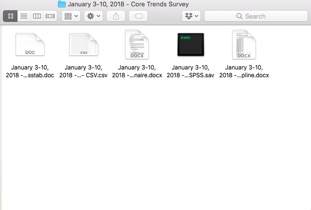
该文件夹包含几种格式的调查数据。就本教程而言, 我们对.csv文件和包含有关调查问卷信息的word文档感兴趣。让我们将数据读入R:
#First, load the following packages (if you don't have them, use the install.packages() function)
library(tidyverse)
library(infer)
#Next, set your working directory to where your Pew data lives, and read it into R
setwd("~/<Your File Path Here>/January 3-10, 2018 - Core Trends Survey")
jan_core_trends_survey <- read_csv("January 3-10, 2018 - Core Trends Survey - CSV.csv")
3.使用整洁的工具进行探索性数据分析
现在我们已经将数据读入R中, 让我们对其进行一些检查:
nrow(jan_core_trends_survey)
length(jan_core_trends_survey)
## [1] 2002
length(jan_core_trends_survey)
## [1] 70
该数据集由2002个观测值组成, 每个观测值都有70个变量。那是大量的变量。现在可能是时候查阅问卷调查表了, 以便更好地了解此调查中记录的数据类型。这是一次电话意见调查, 其中向受访者询问了有关其技术使用和技术观点的一系列问题。还询问了其他有关获取数据的问题, 例如年龄和受教育程度。在问卷中, 提供了与问题相对应的列的名称。例如, 对以下问题的答案:”你是否至少偶尔使用互联网或电子邮件?”存储在eminuse列中。让我们看看它是什么样的:
#what values are stored in the eminuse column?
unique(jan_core_trends_survey$eminuse)
## [1] 1 2 8
#first 10 values of age column
head(jan_core_trends_survey$age)
## [1] 33 76 99 60 55 58
好吧, 这个年龄看起来像我们期望的那样, 但是eminuse列中的值代表什么?
查看调查表, 我们发现有一个对应于值的键, 这些值代表它们所代表的答案:
- 1 =是
- 2 =否
- 8 =(VOL。)不知道
- 9 =(音量)拒绝
eminuse列中的值现在变得更加有意义!现在我们对数据的结构有了更好的了解, 让我们看一下数据集中年龄的分布:
ggplot(jan_core_trends_survey, aes(age)) +
        geom_histogram(bins = 20)

数据集中的年龄分布似乎偏向左侧。考虑总人口中的年龄分布时, 这有意义吗?是!在给定的时间, 较高的人口比例是年轻人, 这与我们上面的直方图一致。
继续前进, 有一系列有趣的列标记为web1a-web1h(例如, web1a, web1b等), 代表受访者对以下问题的回答:”请告诉我你是否在线使用过以下任何社交媒体网站或手机上。”哪里:
- web1a = Twitter
- web1b = Instagram
- web1c = Facebook
- web1d = Snapchat
让我们来探讨一下。这是一个用于计算这些不同社交媒体平台的用户和非用户的平均年龄的函数:
avg_user_ages <- function(df, group, var) {
        #this step is necessary for tidy evaluation
        group <- enquo(group)
        var <- enquo(var)
        df %>%
                select(!!group, !!var) %>%
                ## we are only looking for 1 (user), or 2 (non-user)
                filter(!!group == 1 | !!group == 2) %>%
                group_by(!!group) %>%
                summarize(avg_age = mean(!!var))
}
你可能不熟悉此函数中的某些语法。这是因为dplyr函数使用整洁的评估。在这里可以找到有关阅读更多有关整洁评估工作原理的优秀文档。
使用此功能, 我们看到:
twitter_age <- avg_user_ages(jan_core_trends_survey, web1a, age)

twitter_age
## # A tibble: 2 x 2
##   web1a avg_age
##   <int>   <dbl>
## 1     1    43.3
## 2     2    53.7
instagram_age <- avg_user_ages(jan_core_trends_survey, web1b, age)

instagram_age
## # A tibble: 2 x 2
##   web1b avg_age
##   <int>   <dbl>
## 1     1    40.9
## 2     2    56.2
facebook_age <- avg_user_ages(jan_core_trends_survey, web1c, age)

facebook_age
## # A tibble: 2 x 2
##   web1c avg_age
##   <int>   <dbl>
## 1     1    48.0
## 2     2    58.3
snapchat_age <- avg_user_ages(jan_core_trends_survey, web1d, age)

snapchat_age
## # A tibble: 2 x 2
##   web1d avg_age
##   <int>   <dbl>
## 1     1    35.7
## 2     2    55.9
有趣!也许正如预期的那样, 所有四个平台的用户的平均年龄都大大低于非用户的年龄。对于Snapchat, 平均值相差20年!!
我们可以使用ggplot可视化年龄和Snapchat使用率之间的关系:
#making a dataframe of snapchat users
snap_df <- jan_core_trends_survey %>%
        filter(web1d == 1 | web1d == 2)

#converting the column to a factor, and renaming the factors
snap_df$web1d <- as.factor(snap_df$web1d)
snap_df$web1d <- plyr::revalue(snap_df$web1d, c("1"="user", "2"="non_user"))

#taking a look at the new names
levels(snap_df$web1d)
## [1] "user" "non_user"
#creating and showing a boxplot of ages between users and non-users
snap_age_plot <- ggplot(snap_df, aes(x = web1d, y = age)) +
        geom_boxplot() +
        xlab("Snapchat Usage") +
        ylab("Age")

snap_age_plot

4.使用推断包进行整洁的假设检验
哇, 看起来普通的Snapchat用户比普通的非用户年轻得多。如此巨大的均值差异是由于偶然导致的?让我们进行假设检验!安德鲁·布雷(Andrew Bray)创建了一个很棒的R包来进行整洁的统计推断, 称为推断, 我们之前已经加载了它。该程序包允许指定假设并通过一系列步骤进行测试:1)指定2)假设3)生成4)计算。实际上是这样的:
#first, we calculate and store the observed difference in mean in our dataset
obs_diff <- snapchat_age$avg_age[2] - snapchat_age$avg_age[1]

diff_age_mean <- snap_df %>%
        #specify hypothesis as a formula y ~ x
        specify(age ~ web1d) %>%
        #snapchat usage has no relationship with age
        hypothesize(null = "independence") %>%
        #10, 000 permutations of these data
        generate(reps = 10000, type = "permute") %>%
        #calculate the statistic of interest for the 10, 000 reps
        calculate(stat = "diff in means", order = c("non_user", "user"))

#take a look at the output
head(diff_age_mean)
## # A tibble: 6 x 2
##   replicate   stat
##       <int>  <dbl>
## 1         1 -1.12
## 2         2 -1.53
## 3         3 -1.05
## 4         4  0.516
## 5         5 -1.11
## 6         6  0.332
#how many of the 10, 000 reps are MORE extreme than the observed value?
p <- diff_age_mean %>%
        filter(stat > obs_diff) %>%
        summarize(p = n() / 10000)

p
## # A tibble: 1 x 1
##       p
##   <dbl>
## 1     0
看起来10, 000个均值差异的重复中有0个与观察到的一样极端。我们可以将其解释为意味着观察到的Snapchat使用率和年龄之间的关系确实是偶然的概率极低。但是, 针对年龄之间均值差为0的零假设进行检验并不能单独为我们提供大量信息。如果均值之差不为0, 那是什么?为了回答这个问题, 让我们使用infer构造均值差异的引导置信区间:
age_mean_conf <- snap_df %>%
        #same formula as before
        specify(age ~ web1d) %>%
        #notice that we are now taking the bootstrap rather than permutations
        generate(reps = 10000, type = "bootstrap") %>%
        #Calculate difference in means of each bootstrap sample
        calculate(stat = "diff in means", order = c("non_user", "user"))

#Take a peak at the results of this code
head(age_mean_conf)
## # A tibble: 6 x 2
##   replicate  stat
##       <int> <dbl>
## 1         1  20.6
## 2         2  19.0
## 3         3  19.6
## 4         4  21.1
## 5         5  20.0
## 6         6  19.7
#Now calculate the 95$ confidence interval for the statistic
age_mean_conf %>%
        summarize(lower = quantile(stat, 0.025), upper = quantile(stat, 0.975))
## Response: age (integer)
## Explanatory: web1d (factor)
## # A tibble: 1 x 2
##   lower upper
##   <dbl> <dbl>
## 1  18.4  22.1
我们可以这样解释, 我们有95%的信心Snapchat用户与非用户的平均年龄之间的差异在18.3至22.1岁之间。这是一个有趣的发现!
总结
让我们回顾一下我们所涵盖的内容。首先, 我们获得了有关Pew研究中心以及如何设置Pew帐户以下载其高质量数据的一些背景信息。接下来, 在下载数据之后, 我们看了如何将数据加载到R中并探索其结构。通过R中的数据并了解其基本结构, 我展示了一些简单的可视化如何帮助构建假设以使用数据进行测试。问题是:Snapchat用户和非用户的平均年龄有何不同?这个问题是使用infer包编码的。我们了解到, Snapchat用户的平均年龄比未使用该平台的用户低18.3至22.1岁!
这就是本教程的全部内容!我希望你喜欢从Pew研究中心浏览有关社交媒体使用情况的数据, 并鼓励你浏览更多有关其真棒数据并查看可以找到的内容。编码愉快!
如果你想了解有关R的更多信息, 请参加srcmini的Data.table Way课程R中的数据分析。
评论前必须登录!
注册