Tidyverse足球得分分析

本文概述

• 当苏格兰足球遇上tidyverse
• 整理时间

在本教程中，我们将使用tidyr、dplyr和ggplot2来可视化一个赛季的足球比分，并研究进球和失球时间的趋势。

当苏格兰足球遇上tidyverse

我整理了当地足球队的一些数据, 我们可以使用tidyverse的工具来练习一些数据重塑技术。

重构数据后, 我们将绘制其2017/2018联赛运动的每场比赛的每个进球。目的是创建一个图, 其中每个方面都显示进球和失球的时间轴。

我们将使用tidyr, dplyr和ggplot2来创建主要图形, 并绘制一些图表来查看进球和失球时的趋势。

(可选)我们可以使用开发中的” gganimate”包对最终图形进行动画处理。

这个想法的灵感来自(但绝非要直接复制)数据可视化大师Andy Kirk的工作, 他几年前对利物浦足球俱乐部的赛季进行了可视化(http://www.visualisingdata.com/2016/ 05 /臂架形状辊过山车季节/)。

那个赛季在红军的欧洲决赛中结束。

我的团队是位于苏格兰高地的因弗内斯加里东尼亚蓟FC。去年, 他们的目标是升职回到苏格兰超级联赛, 此前他们降级了。让我们看看这是否是图卢克喀里多尼亚体育场的过山车季节。

原始数据存储在excel工作簿中, 因此, 除了加载tidyverse程序包外, 我们还将使用readxl程序包导入数据。

让我们加载所需的包, 然后读取数据。

library(readxl)
library(tidyverse)
scores <- read_excel("InvernessResults2017.xlsx", sheet = "scores")

这是电子表格数据的链接。

让我们看一下数据。

glimpse(scores)

“结果”列告诉我们因弗内斯赢了, 输了还是比赛是平局。

我们有”主场”球队得分和”客场”球队得分的列, 以及指示因弗内​​斯是主场还是客场的列。通常情况下, 球队会交替比赛, 但有时也会进行一些主场比赛, 反之亦然。绘制图时, 我们总是希望Inverness得分首先出现, 因此我们需要找出一种方法来使Result列的顺序保持一致。

我们可以看到对方球队的名字：

unique(scores$Opponent)

联赛中有10支球队, 每支球队与其他球队进行4场比赛(主场2场, 客场2场), 因此, 总共36场。

我们为每支球队的得分提供了一个专栏, 其他专栏则显示了每个进球的时间。

例如, 如果Inverness得分为3个目标, 则Inv_Goal_1, Inv_Goal_2和Inv_Goal_3列将具有条目, 而Inv_Goal4和Inv_Goal5列将保持为NA。

我们一定会浓缩这些专栏。

在此之前, 我们将创建一个用于绘制目的的辅助数据框。稍后我们可以使用它来加入分数数据框架。

team <- c('Brechin', 'Dumbarton', 'Dundee_United', 'Dunfermline', 'Falkirk', 'Greenock_Morton', 'Inverness', 'Livingston', 'Queen_Of_The_South', 'St_Mirren')
colors <- c('#E3001B', '#F8BE02', '#C6631D', '#161616', 'midnightblue', '#316891', '#0355AF', '#C19B24', '#093C71', '#000000')


team_df <- tibble(team, colors)

rm(list = c("colors", "team"))

颜色已被选为与每个团队的比赛工具包中的主要颜色最匹配的颜色(不要太着迷)。

整理时间

好了, 足够的序言, 让我们看看我的团队是如何做的…

首先, 数据框中的列名称均以大写字母开头。这可能会有问题, 所以让我们将它们更改为小写：

colnames(scores) <- colnames(scores) %>% str_to_lower()

这样更好现在, 使用tidyr的gather函数处理所有显示每个目标时间的列。

首先, 我们选择日期列, 所有以” inv”开头的列以及以” opp”开头的列。我们还将选择” gameid”列以用于计算将来的变量。

看一下”聚会”电话。我们将获取所有目标列, 并将其转换为一个长列, 称为”目标”(由’key’参数定义)。除此之外, 我们还创建了一个新的长列, 称为”时间”, 在其中计入了目标时间的所有值。我们选择的所有其他列也以”长”格式存储。

data <- scores %>%
  select(date, starts_with("inv"), starts_with("opp"), gameid) %>%
  gather(inv_goal_1, inv_goal_2, inv_goal_3, inv_goal_4, inv_goal_5, opp_goal_1, opp_goal_2, opp_goal_3, opp_goal_4, opp_goal_5, key = "goal", value = "time")

让我们看一下这个新的数据框：

str(data)

我们的”分数”数据帧长36行, 宽20列。现在, 我们的”聚集”数据帧的长度为360行, 但宽度仅为8列。

我们将再添加一列, 以供日后对图进行分面时使用。

data <- data %>%
mutate( result = paste(inverness_score, "-", opponent_score))

我们需要在其中添加一个”团队”列, 此外, 我们还需要按比赛逐个团队获取每个目标的累计计数。

plot_data <- data %>%
   select(date, opponent, gameid, goal, time, result, inverness_status) %>%
  mutate(team = if_else(str_sub(goal, 1, 1) == "i", "inverness", tolower(opponent))) %>%
  group_by(gameid, team) %>%
  arrange(time) %>%
  mutate(count = 1) %>%
  ungroup() %>%
  group_by(gameid, team) %>%
  mutate(goalcount = cumsum(count)) %>%
  ungroup() %>%
  select(-count)

我们将为每个目标使用geom_rect()。这需要沿x和y轴的最小值和最大值。我们将使用dplyr的lag和Lead函数创建这些值。例如, 得分的第二个目标将具有等于第一个目标的时间的最小值, 而最大值将是第二个目标的实际时间。同时, 最小y值为1, 最大y为2。

当我们制作剧情时, 它将变得更加清晰！

plot_data <- plot_data %>%
  group_by(gameid) %>%
  arrange(gameid, time) %>%
  mutate(lag_time = lag(time), lead_time = lead(time)) %>%
  ungroup()

plot_data$lag_time[is.na(plot_data$lag_time)] <- 0

plot_data$lead_time[is.na(plot_data$lead_time)] <- 90

后两个命令分别将滞后时间和提前时间中的NA分别替换为0和90。现在, 我们以所需顺序选择所需的列。

plot_data <-  plot_data %>%
  select(gameid, date, team, result, opponent, goalcount, lag_time, time, lead_time, inverness_status)

我们要确保我们保留那些以0-0无得分结束的比赛的行。否则, 这些结果将从最终绘图中删除。

goalless <- filter(plot_data, result == "0 - 0")

但是, 我们不需要其他游戏中没有”时间”价值的多余行。因此, 我们将其过滤掉, 然后合并两个数据框, 并保留plot_data名称。

scored <- filter(plot_data, result != "0 - 0") %>%
  filter(!is.na(time))

plot_data <- bind_rows(goalless, scored)

rm(list = c("goalless", "scored"))

现在终于可以绘制了。你可能想要为此最大化绘图窗口。

p <- ggplot(plot_data, aes(time, goalcount, group = opponent, fill = team)) +
  geom_rect(aes(xmin = lag_time, xmax = time, ymin = (goalcount - 1), ymax = goalcount)) +
  geom_text(aes(x = 25, y = 4.5, label = result , size = 0.5)) +
theme_void() +
  scale_fill_manual(values = team_df$colors) +
  facet_wrap(date + inverness_status ~ opponent, ncol = 9) +
  ggtitle(label = "Inverness Caledonian Thistle Goals Scored / Conceded - Scottish Championship 2017/2018") +
  labs(x = NULL, y = NULL) +
  theme(legend.position = "none")
print(p)

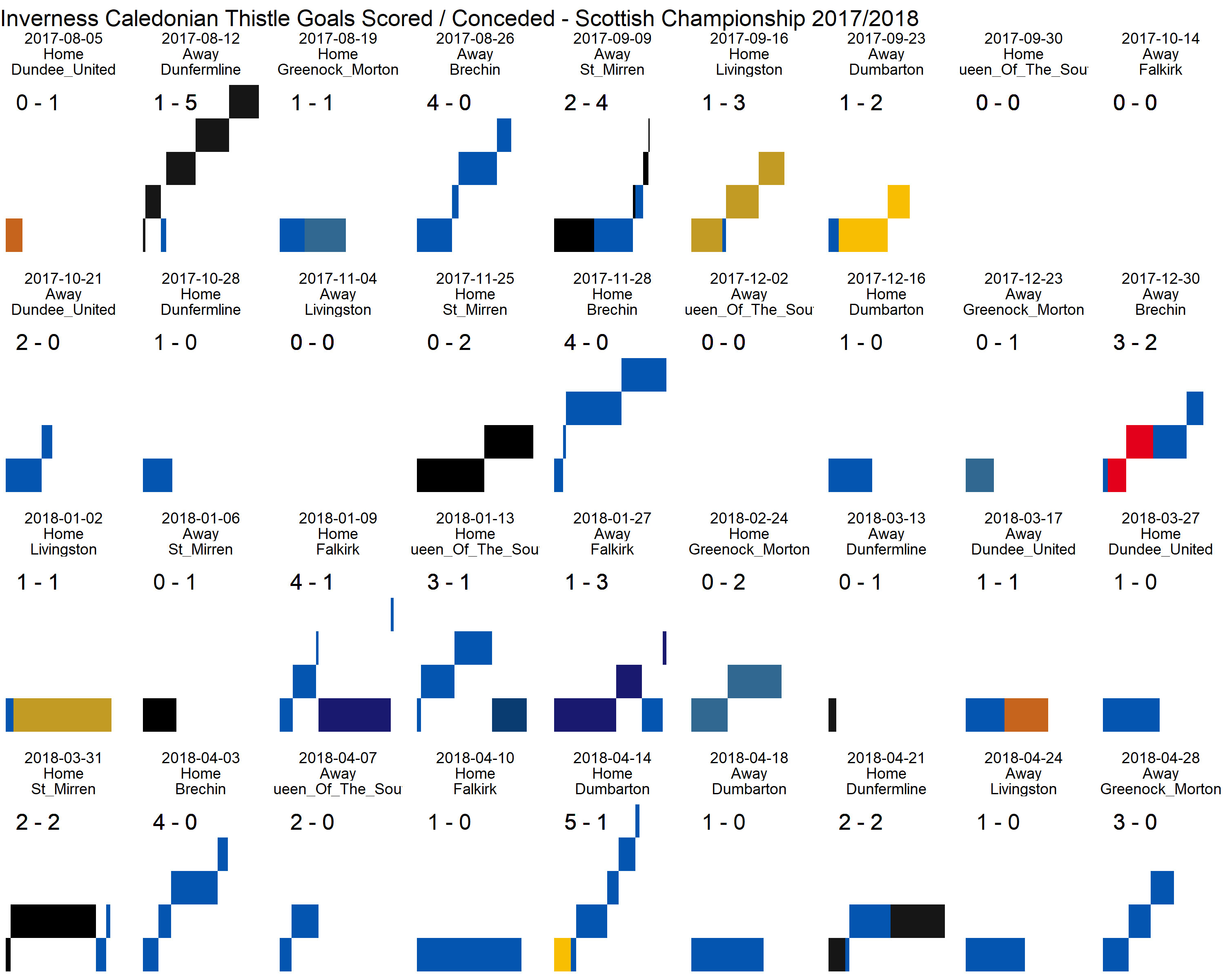
接下来, 你将找到每场比赛进球进球的时间表。

在获得这些数据的同时, 我们也可能希望查看团队得分或失球的时间是否有任何规律。由于每场比赛持续90分钟(不包括停赛所需的时间), 因此我们可以查看以15分钟为间隔的进球数。

plot_data$cut <- cut(plot_data$time, seq(0, 90, by = 15))

inv_scored <- plot_data %>%
  filter(team == "inverness", !is.na(time))

  ggplot(inv_scored, aes(goalcount, time, group = goalcount)) +
  geom_boxplot(width = 0.2) +
  geom_point() +
  ggtitle(label = " When Inverness goals 1 to 5 are scored - by minute of match") +
  scale_y_continuous(breaks = seq(0, 90, by = 15)) +
  theme_bw()

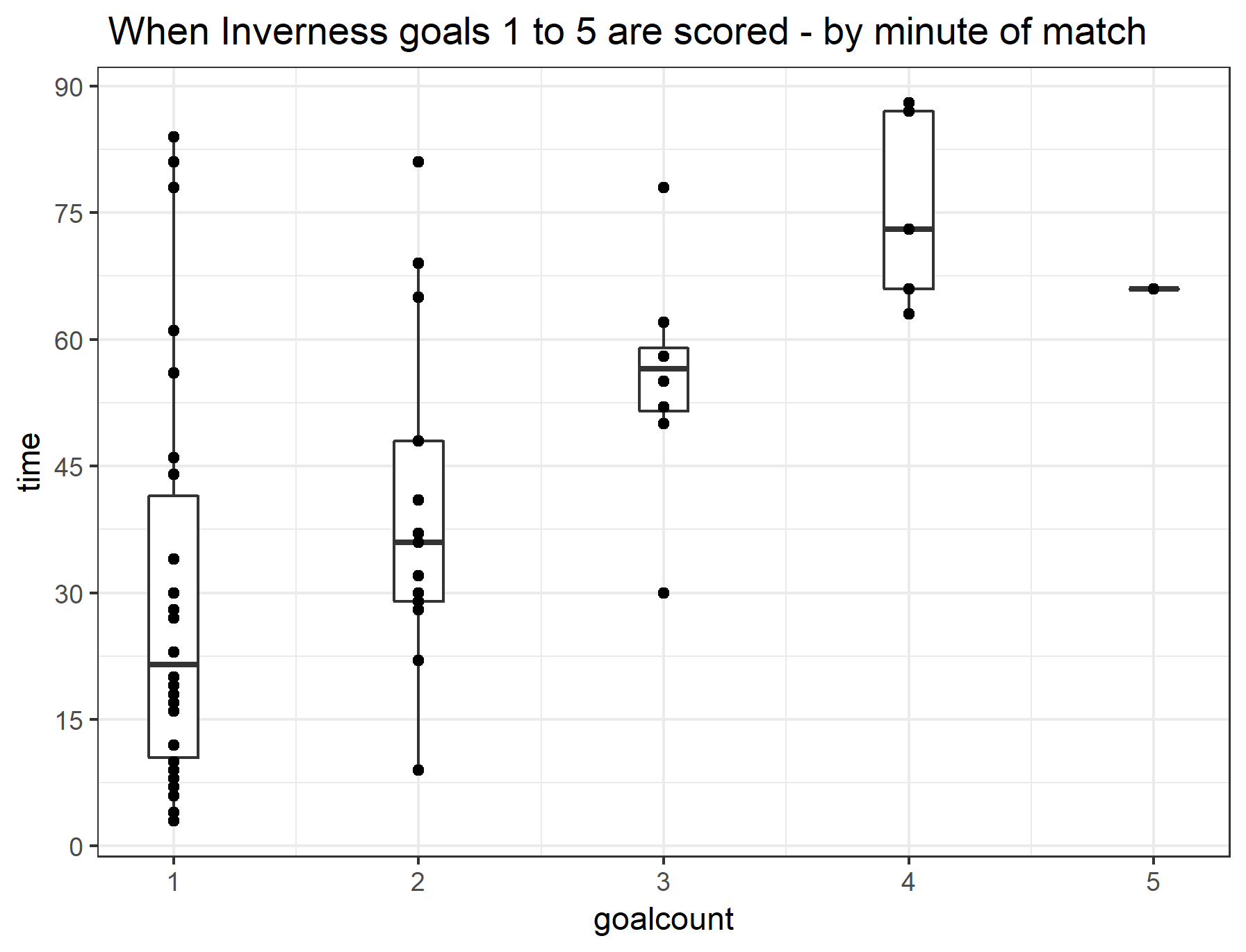
看来球队在前30分钟内经常得分1或2个进球(尽管这与我对比赛的记忆没有关系)。

对手中的任何一支球队特别容易在比赛开始时就让他们进球吗？

opposing_colors <- team_df %>% filter(team != "Inverness")

ggplot(inv_scored, aes(goalcount, time , group = goalcount, fill = opponent)) +
  geom_boxplot(width = 0.2) +
  ggtitle(label = "Inverness goals scored by opponent and minute of match") +
  scale_y_continuous(breaks = seq(0, 90, by = 15)) +
  facet_wrap(~ opponent) +
  theme_bw() +
  theme(legend.position = "bottom") +
  scale_fill_manual(values = opposing_colors$colors)

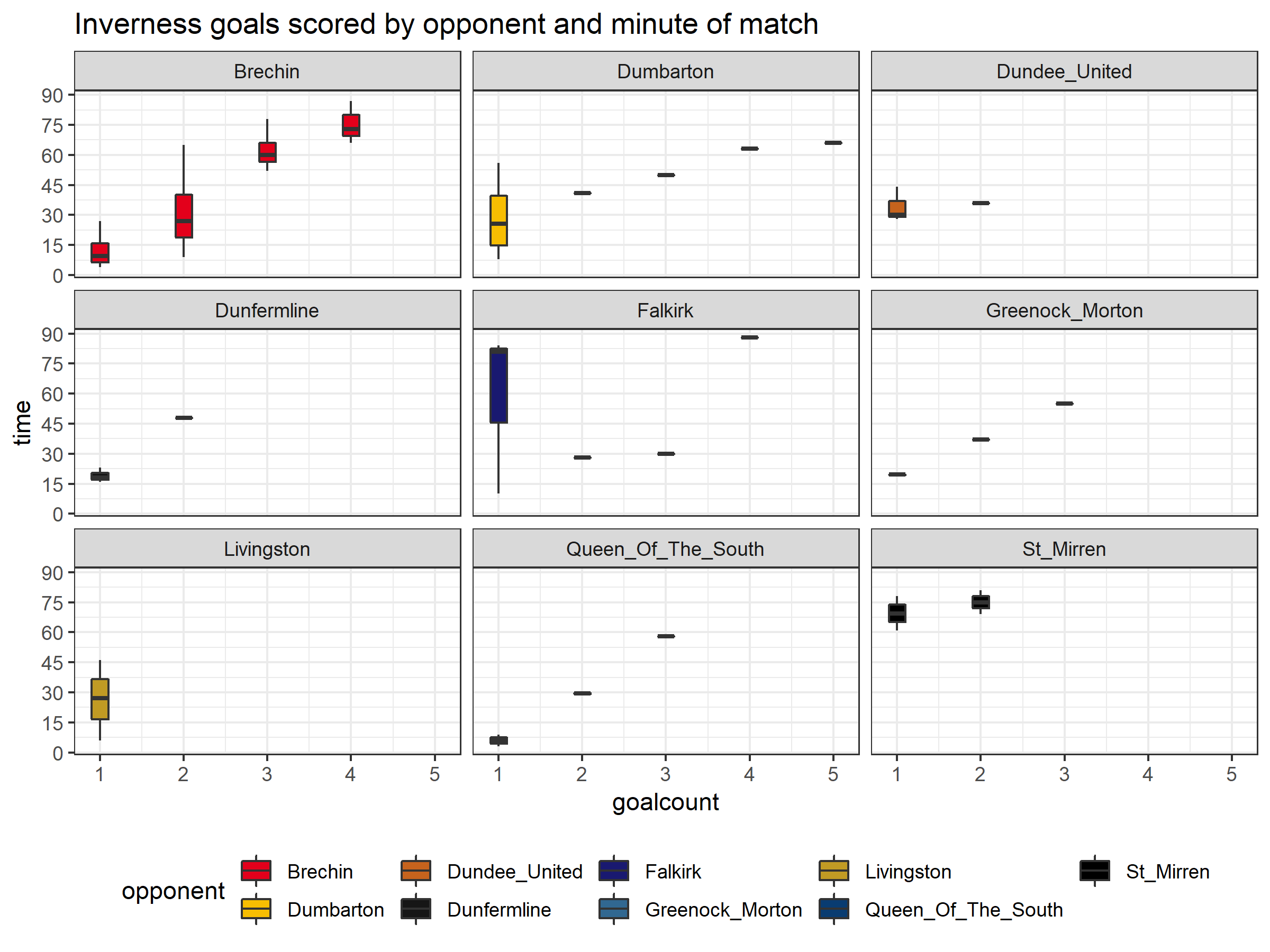
因此, 看来球队在与布雷钦, 邓巴顿和利文斯顿的比赛中得分较高。

当然, 我们也可以为所承认的目标做同样的事情：

ggplot(opposition_score, aes(goalcount, time, group = goalcount)) +
  geom_boxplot(width = 0.2) +
  geom_point() +
    ggtitle(label = "Inverness goals conceded by minute of match") +
  scale_y_continuous(breaks = seq(0, 90, by = 15)) +
  theme_bw()

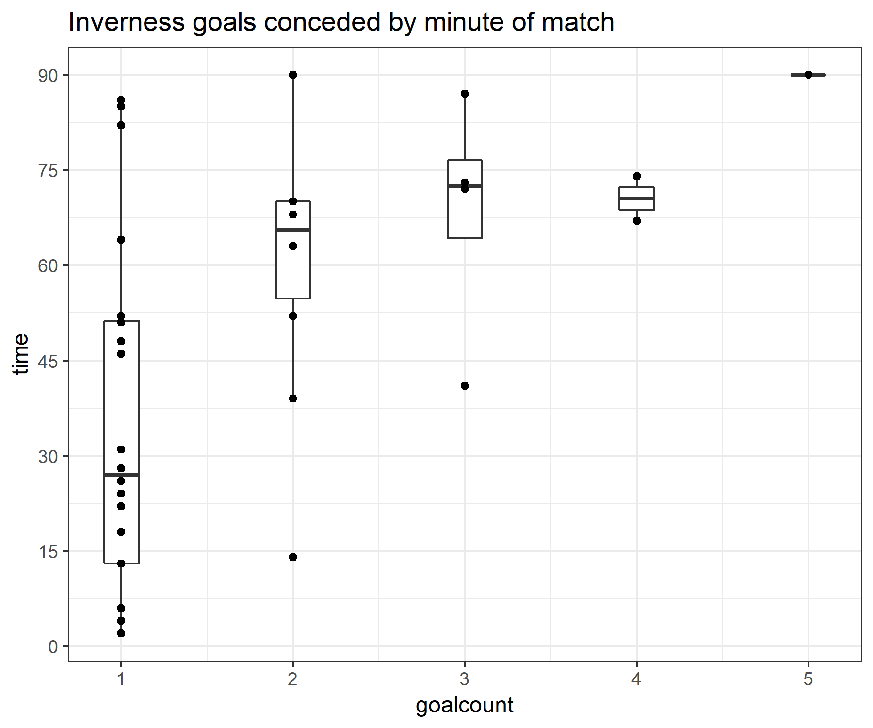
好吧, 这很有趣, 因为如果因弗内斯认输2个或更多进球, 通常会在比赛的下半场发生。

进球和失球的时间之间是否存在统计差异？我们可以使用ggplot2来提供帮助。

comparison <- plot_data %>%
  select(team, goalcount, time) %>%
  filter(!is.na(time)) %>%
  mutate(team_type = if_else(str_sub(team, 1, 1) == "i", "Inverness", "Opponent"))

ggplot(comparison, aes(team_type, time, group = team_type, fill = team_type)) +
geom_boxplot(width = 0.2, notch = TRUE) +
    ggtitle(label = "Distribution of time of nth goal scored / conceded by minute of match") +
  theme_minimal() +
  scale_y_continuous(breaks = seq(0, 90, by = 15)) +
  theme(legend.position = "bottom") +
  scale_fill_manual(values = c('#0355AF', '#E3001B')) +
  facet_wrap(vars(goalcount), ncol = 3)

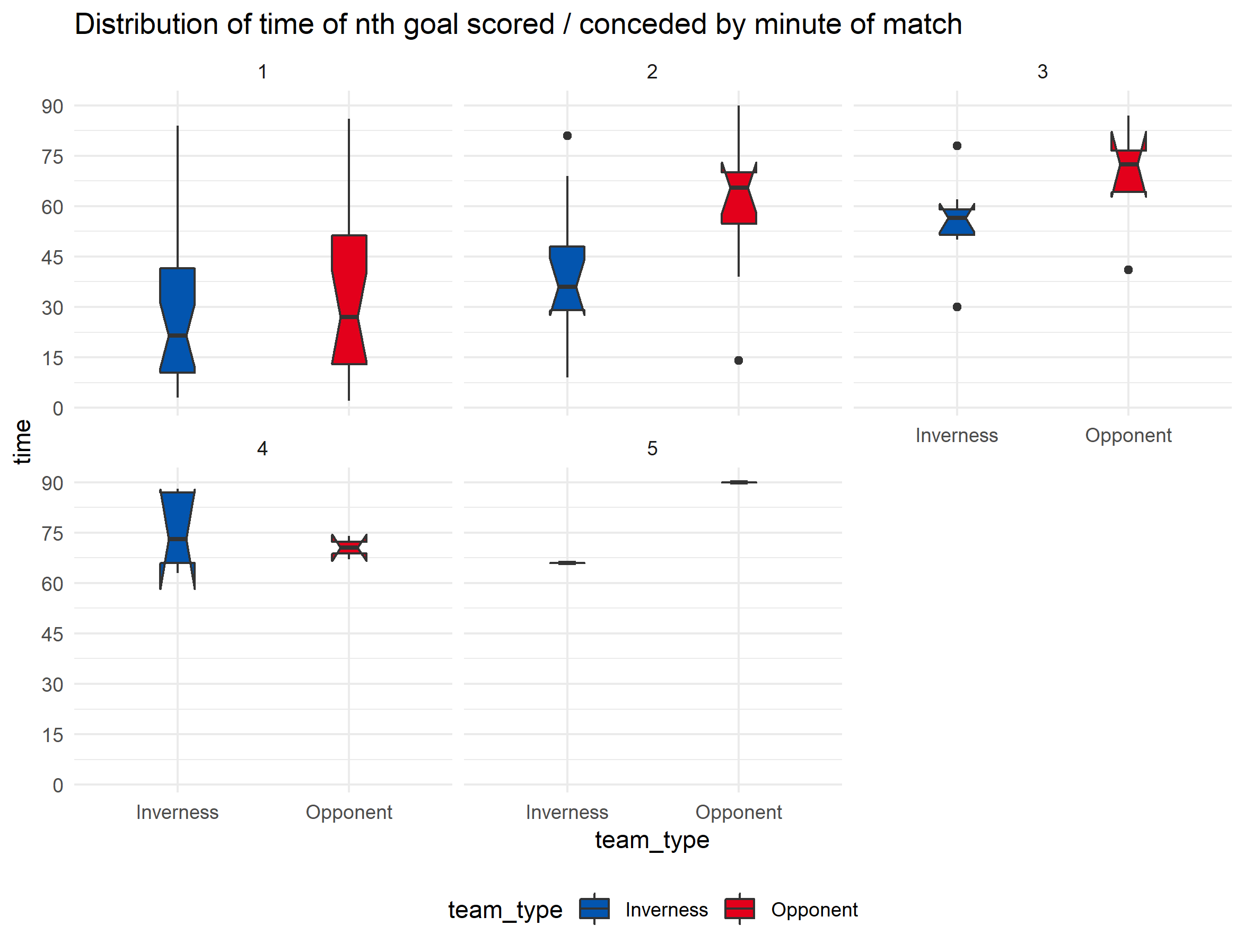
尽管可能很难看到, 但取决于你的绘图窗口, 第二个和第三个目标的箱形图上的凹口不会重叠。这表明存在统计学差异-因弗内斯很可能比他们承认的更早获得第二个进球, 同样, 第三个进球也是如此。进球5也不存在任何重叠, 但是因为在比赛中得分5或让其失球是罕见的, 所以我们可以忽略这一点。

动画情节

最后-尽管我们之前创建的目标时间线图与Andy Kirk的原始图形不太一样, 但我们仍然可以从中获得乐趣。

N.B-这是可选的, 需要从github安装最新版本的gganimate。

如果这不可能, 请不要担心, 因为最终输出将显示在下面, 因此你可以看到会发生什么。

另请注意-创建此动画可能需要几分钟。

# gganimate is currently in development on github
# You will need to install devtools if you haven't already done so
# You will require to be using the latest version of R and may need to reinstall your existing packages.


# install.packages('devtools')
#devtools::install_github('thomasp85/gganimate')

library(gganimate)

#we already defined p as our original season plot
# but we will rebuild it here  just in case you have removed it from your workspace
p <- ggplot(plot_data, aes(time, goalcount, group = opponent, fill = team)) +
  geom_rect(aes(xmin = lag_time, xmax = time, ymin = (goalcount - 1), ymax = goalcount)) +
  geom_text(aes(x = 25, y = 4.5, label = result , size = 0.5)) +
theme_void() +
  scale_fill_manual(values = team_df$colors) +
  facet_wrap(date + inverness_status ~ opponent, ncol = 9) +
  ggtitle(label = "Inverness Caledonian Thistle Goals Scored / Conceded - Scottish Championship 2017/2018") +
  labs(x = NULL, y = NULL) +
  theme(legend.position = "none")
print(p)

# now we take the previous plot, and animate it using the game id to render each faceted plot, in date order
# q <- p + transition_states(gameid, transition_length = 1, state_length = 1) + shadow_mark(past =  TRUE) # this ensures all previous plots are shown
# animate(q, width = 900, height = 750)

#anim_save("game_by_game_season_plot.gif")

在本赛季糟糕的开局之后(该队排名第9位), 他们逐渐开始获得动力。联赛中有几场杯赛, 在此期间他们设法创造了俱乐部纪录, 记录了每分钟上场比赛的次数。

如果联盟在一月份开始, 他们将是冠军。

事实如此, 直到赛季结束, 他们一直保持不败的状态, 他们赢得了Irn Bru杯冠军(这要归功于加时赛冠军), 而且他们在晋级附加赛中的表现也差强人意。

最终, 他们被邓弗姆林(Dunfermline)撤消, 后者在联赛中保持不败, 并且至关重要的是, 在本赛季的最后一场”必赢”主场比赛中, 他们获得了第96分钟的扳平比分, 但仅获得第四名。

但是, 随着球队现在已经适应了冠军联赛, 一些新的签约, 以及与他们新近降级的本地对手至少进行了4场比赛, 新赛季还有很多值得期待的事情。

如果你想了解有关Tidyverse的更多信息, 请参加以下srcmini课程：

• Tidyverse简介
• Tidyverse中的分类数据
• 在Tidyverse中处理数据
• 在Tidyverse中与数据进行通信
• 在Tidyverse中使用数据建模